Project page: http://rncarpio.github.com/delaunay_linterp
What is delaunay_linterp?
delaunay_linterp is a C++ header-only library for N-dimensional piecewise linear interpolation of unstructured data, similar to Matlab's
griddata and SciPy's griddata commands. Suppose we are given a set of data
points (x, f(x)) where x is N-dimensional. The idea is to construct an N-dimensional Delaunay triangulation of the x coordinates of the data points; each vertex in the triangulation corresponds to a data point (x, f(x)). To compute an interpolated value for xi, we:
- locate the simplex containing
xi - calculate the barycentric coordinates of
xiin the simplex - calculate
interp(xi)as a weighted sum of the values off(x)at the vertices of the simplex
The interpolated surface is linear within each simplex of the triangulation.
The CGAL computational geometry library is used for the underlying triangulation code. Other libraries that are used are:
- Boost - C++ libraries
- GMP - arbitrary precision arithmetic (on Windows, MPIR is used)
- MPFR - multi-precision floating point
- Eigen - C++ linear algebra
Points can be added incrementally. In addition, a function specifying f(x) can be passed to the triangulation. delaunay_linterp can adaptively choose where to insert data points, by maintaining a list of approximation errors associated with each simplex of the triangulation. This allows a good approximation of arbitrary functions with few data points, compared to regular grids.
dD vs. 2D
CGAL has more than one package for constructing a Delaunay triangulation:
- a d-dimensional library that uses the lifting transform, then constructs a convex hull in d+1 dimensions. This is very flexible and can handle arbitrary dimensions, but it is much slower than the libraries specifically designed for 2D and 3D.
- 2D and 3D specific libraries which are much faster.
delaunay_linterp provides classes using the dD and 2D libraries (3D coming soon...).
- for dD, use the
delaunay_d_interpclass. Caveats: currently, it cannot handle interpolation queries outside the convex hull of the inserted points - for 2D, use the
delaunay_2_interpclass
C++ interface
Here is an example in C++:
#include <ctime>
#include "delaunay_2_interp.h"

// return an evenly spaced 1-d grid of doubles.
std::vector<double> linspace(double first, double last, int len) {
  std::vector<double> result(len);
  double step = (last-first) / (len - 1);
  for (int i=0; i<len; i++) { result[i] = first + i*step; }
  return result;
}

// the function to interpolate.
double fn (double x1, double x2) { return pow(x1,0.3) * pow(x2,0.6); }

int main(int argc, char **argv) {
  int n_points = 10;
  clock_t t1, t2;

  // first, try a rectangular grid
  Delaunay_incremental_interp_2 triang;
  std::vector<double> grid = linspace(0., 5., n_points);
  t1 = clock();
  for (int i=0; i<n_points; i++) {
    for (int j=0; j<n_points; j++) {
      array<double,2> args = {grid[i], grid[j]};
      triang.insert(args.begin(), args.end(), fn(args[0], args[1]));
    }
  }
  t2 = clock();
  printf("regular grid: %d insertions, %d clocks, %f sec\n", n_points*n_points, (t2-t1), ((double)(t2 - t1)) / CLOCKS_PER_SEC);

  // second, try adaptive point placement
  std::function<double(double, double)> fn_obj(fn);
  Delaunay_incremental_interp_2 adaptive_triang(fn_obj);
  // insert boundary points
  array<double,2> args;
  t1 = clock();
  args[0]=grid.front(); args[1]=grid.front();   adaptive_triang.insert(args.begin(), args.end(), fn(args[0], args[1]));
  args[0]=grid.front(); args[1]=grid.back();    adaptive_triang.insert(args.begin(), args.end(), fn(args[0], args[1]));
  args[0]=grid.back(); args[1]=grid.front();    adaptive_triang.insert(args.begin(), args.end(), fn(args[0], args[1]));
  args[0]=grid.back(); args[1]=grid.back();     adaptive_triang.insert(args.begin(), args.end(), fn(args[0], args[1]));
  for (int i=0; i<n_points*n_points-4; i++) {
    adaptive_triang.insert_largest_error_point();
  }
  t2 = clock();
  printf("adaptive grid: %d insertions, %d clocks, %f sec\n", n_points*n_points, (t2-t1), ((double)(t2 - t1)) / CLOCKS_PER_SEC);

  // compare interpolated value vs. actual function
  std::vector<double> true_f_vals, interp_grid = linspace(0., 5., 2*n_points);
  for (int i=0; i<interp_grid.size(); i++) {
    for (int j=0; j<interp_grid.size(); j++) {
      array<double,2> args = {interp_grid[i], interp_grid[j]};
      true_f_vals.push_back(fn(args[0], args[1]));
    }
  }

  // get the interpolated values
  std::vector<double> regular_triang_vals, adaptive_triang_vals;
  t1 = clock();
  for (int i=0; i<interp_grid.size(); i++) {
    for (int j=0; j<interp_grid.size(); j++) {
      array<double,2> args = {interp_grid[i], interp_grid[j]};
      regular_triang_vals.push_back(triang.interp(args.begin(), args.end()));
    }
  }
  t2 = clock();
  printf("regular grid: %d interpolations, %d clocks, %f sec\n", regular_triang_vals.size(), (t2-t1), ((double)(t2 - t1)) / CLOCKS_PER_SEC);
  t1 = clock();
  for (int i=0; i<interp_grid.size(); i++) {
    for (int j=0; j<interp_grid.size(); j++) {
      array<double,2> args = {interp_grid[i], interp_grid[j]};
      adaptive_triang_vals.push_back(adaptive_triang.interp(args.begin(), args.end()));
    }
  }
  t2 = clock();
  printf("adaptive grid: %d interpolations, %d clocks, %f sec\n", adaptive_triang_vals.size(), (t2-t1), ((double)(t2 - t1)) / CLOCKS_PER_SEC);

  // compute sum of squared errors
  double sse1=0.0, sse2=0.0, diff;
  for (int i=0; i<true_f_vals.size(); i++) {
    diff = true_f_vals[i] - regular_triang_vals[i];
    sse1 += diff*diff;
    diff = true_f_vals[i] - adaptive_triang_vals[i];
    sse2 += diff*diff;
  }
  printf("regular grid: sum of squared errors: %f\n", sse1);
  printf("adaptive grid: sum of squared errors: %f\n", sse2);

  return 0;
}
produces:
regular grid: 100 insertions, 6 clocks, 0.006000 sec
adaptive grid: 100 insertions, 11 clocks, 0.011000 sec
regular grid: 400 interpolations, 2 clocks, 0.002000 sec
adaptive grid: 400 interpolations, 2 clocks, 0.002000 sec
regular grid: sum of squared errors: 5.800002
adaptive grid: sum of squared errors: 0.044019
Python interface
A Python interface is provided, using Andreas Klöckner's pyublas library. Pre-built binaries are in the windows_binaries directory; these were built against PythonXY version 2.7.3.1.
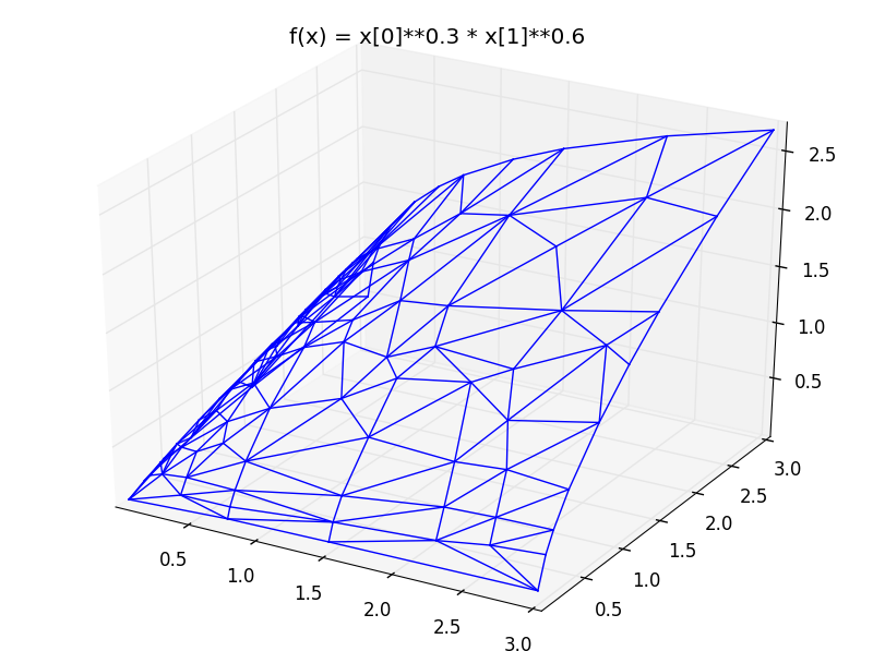
Example:
import scipy
import matplotlib.pyplot as plt
from mpl_toolkits.mplot3d import Axes3D
import _delaunay_2_python as _delaunay2

def plot_triang_2d(triang, title=None, show_concave=False):
    fig = plt.figure()
    ax = Axes3D(fig)
    (all_segments, min_coords, max_coords) = triang.get_line_segments()

    for segment in all_segments:
        (p0, p1, is_concave) = segment
        if (show_concave):
            color = ('b' if (is_concave) else 'r')
        else:
            color = 'b'
        (xpair, ypair, zpair) = zip(p0, p1)
        ax.plot3D(xpair, ypair, zpair, color=color)
    ax.set_xlim(min_coords[0], max_coords[0])
    ax.set_ylim(min_coords[1], max_coords[1])
    ax.set_zlim(min_coords[2], max_coords[2])
    if (title != None):
        ax.set_title(title)
    return ax

# the function to be approximated
def fn(x):
    return x[0]**0.3 * x[1]**0.6

# create triangulation object
triang = _delaunay2.DelaunayInterp2(fn)

# insert boundary points
for x in [ [0.01, 0.01], [0.01, 3.0], [3.0, 0.01], [3.0, 3.0] ]:
    triang.insert(x, fn(x))

# adaptively place points
for i in range(100):
    triang.insert_largest_error_point()

# plot triangulation
plot_triang_2d(triang, title="f(x) = x[0]**0.3 * x[1]**0.6")
produces
License: GPLv3
delaunay_linterp is free software: you can redistribute it and/or modify it under the terms of the GNU General Public License as published by the Free Software Foundation, either version 3 of the License, or (at your option) any later version.
This program is distributed in the hope that it will be useful, but WITHOUT ANY WARRANTY; without even the implied warranty of MERCHANTABILITY or FITNESS FOR A PARTICULAR PURPOSE. See the GNU General Public License for more details.
You should have received a copy of the GNU General Public License along with this program. If not, see http://www.gnu.org/licenses/.